Scaling of Ecosystem Services
![]()
NSERC ResNet HQP Scaling Group
Introduction
Different scale(s) are most meaningful for a given decision or research question
We design studies at different scales, because
(1) decision-makers require data at different spatio-temporal scales and
(2) scientists seek to understand how ecosystem processes and properties vary across scales.
There are cost and time constraints to collecting data; therefore, we target the scale most relevant for a given question or decision.
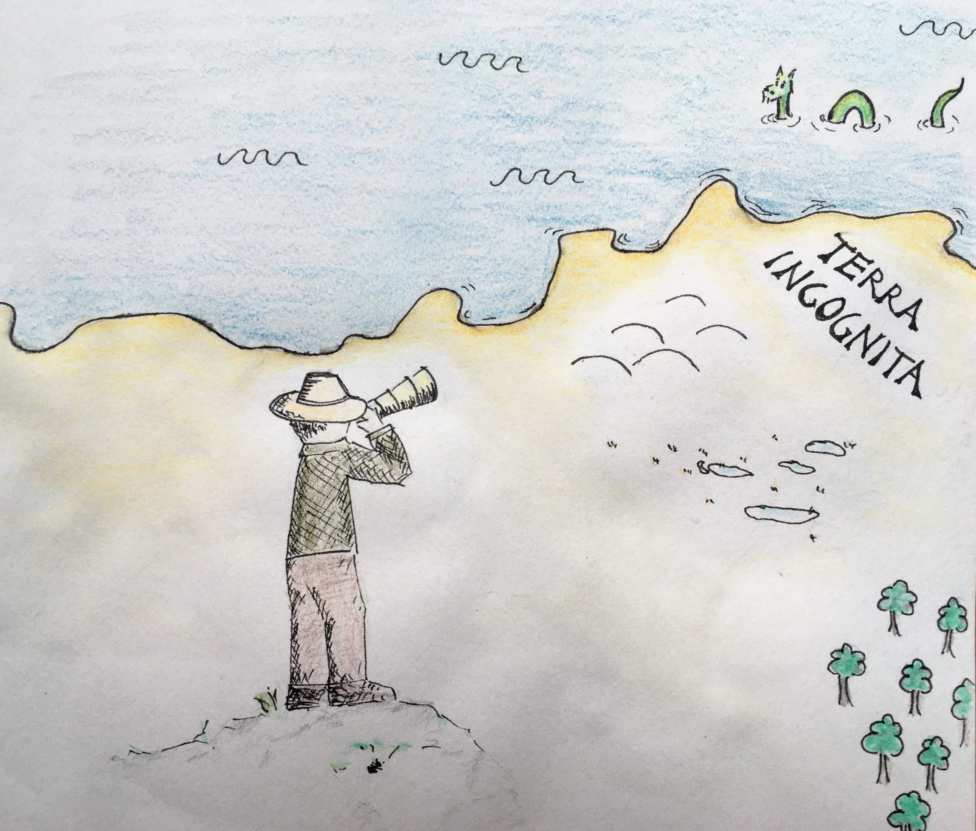


*Created by Ágnes Vári. The idea behind this drawing is to start as a decision-maker, researcher, and/or explorer, and show how the view (scale) may change, in a fun way, before we dive into the scientific details. We will finish this sketch after the AGM. *
Defining terms
[Placeholder text: We plan to hire an illustrator to create a visual defining the terms: ecosystem service, supply, demand, flow, benefit, etc. There will be one hexagon at a landscape scale and a second hexagon nested behind at a regional scale. We will also add a glossary section for readers to find more information on the terms used in this story map.]
Changing spatial and temporal scales
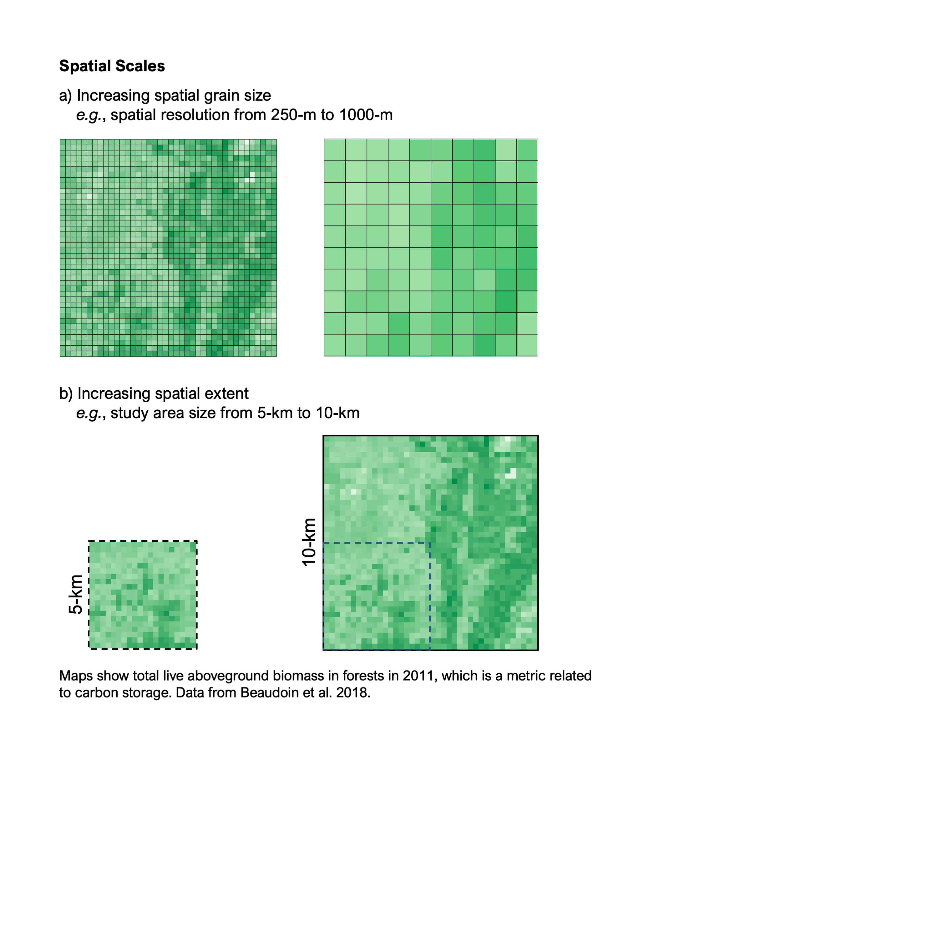
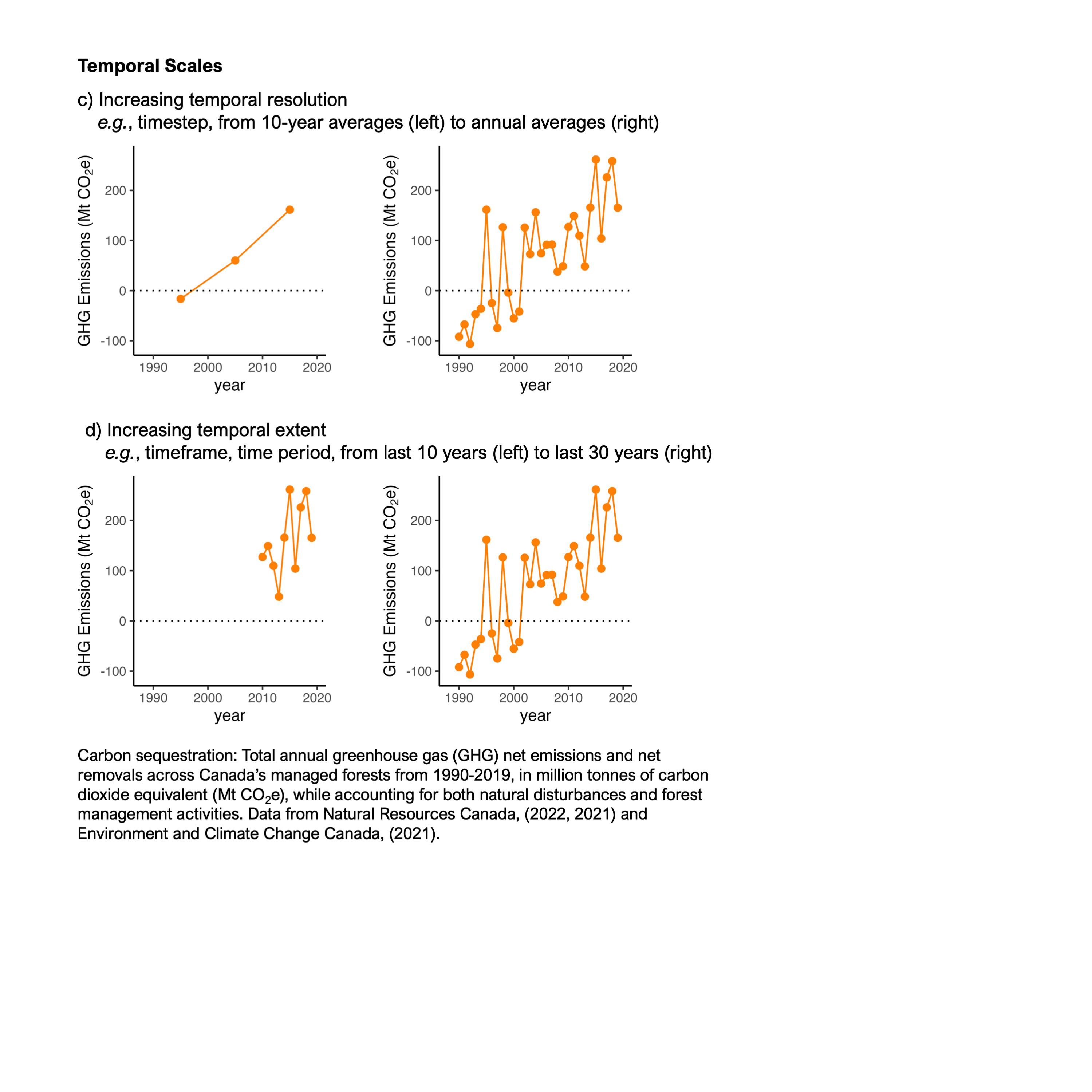
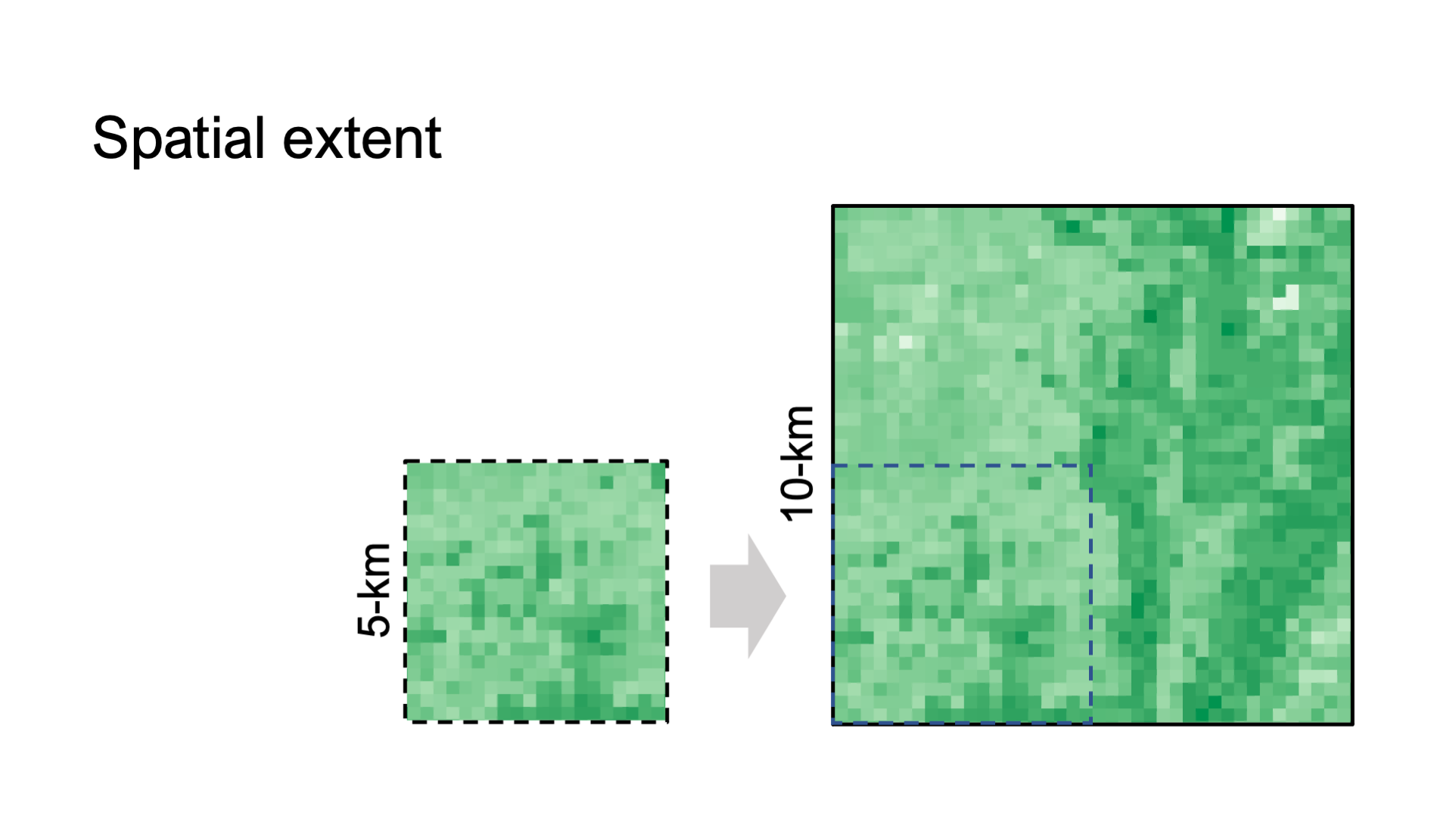
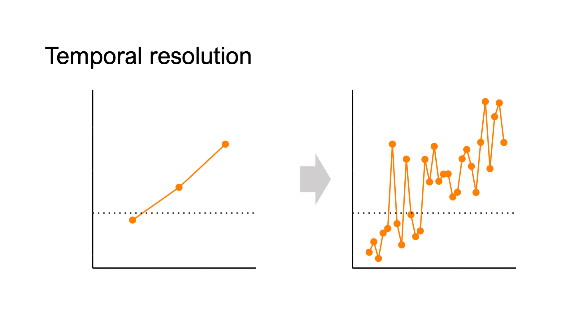
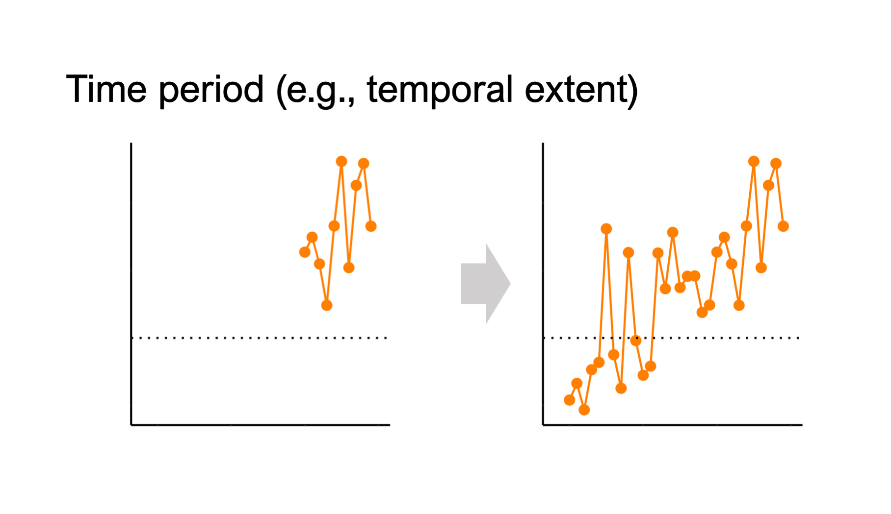
Often data is only available (or can only be collected) at one scale; however, we need information at a different scale to inform a decision or to understand an ecological process. In the figure below we visualize what it means to increase (a) spatial grain size, (b) spatial extent, (c) temporal resolution, and (d) time period.
Why do we scale up or down?
We may scale up or down for many reasons, including these examples:
-
It can be expensive, time-consuming, and dangerous to collect data points in the field at every possible location. Instead, we stratify (e.g., partition) a larger landscape into smaller homogenous areas and take representative samples within each group.
-
Ecological processes can be difficult to observe directly, including when processes are too fast, too slow, too small, or too large. We develop models to visualize a reality that is inaccessible to our senses.
-
Management and policy decisions may require data at a different scale (e.g., extent or grain) compared to the scale of available data. For example, we may collect field data about a management intervention at a local scale; however, we may rely on models to test how scaling these interventions could affect outcomes at a larger scale.
-
There are many decision-makers at different (nested) spatial scales, with their own mandates, agendas, and actions. Land-use planning policies are often developed considering scales that represent political needs at regional scales, which may or may not be consistent with ecological and societal needs at local scales. For example, climate change mitigation actions at a national scale, may not address heterogeneous needs at finer scales, for example cooling effects at the neighborhood scale.
As a part of ResNet we research these scaling topics
What is ResNet?
We are part of the ResNet network that unites a broad community of scholars, NGO, government, and industry sectors. We are based in different working landscapes across Canada, and our aim is to improve our capacity to monitor, model, and manage these landscapes and all the ecosystem services that they provide for long-term well-being and shared prosperity.
Introduction to the process of creating this story map
Together as students and postdocs within the multi-scale ResNet network, we discuss a few of the challenges and best practices related to scaling. [Add link to who we are? section].
For more information about ResNet click here
Shared challenges
In the next sections, we discuss a few of the challenges related to scaling of ecosystem services and best practices for overcoming these challenges.
We use case studies to illustrate each challenge. Icons at the top right illustrate whether the case study focuses on scaling challenges related to changing (a) spatial grain size, (b) spatial extent, (c) temporal resolution, and (d) time period
Challenge: Field work is critical
[under construction note]
Introduction
[This section is under construction and will be updated after the AGM; however, we provide notes of our current thoughts]
There is a trade-off between the need for field data but the time and funding needed to collect and process field samples. When collecting samples in the field it is important to consider…
- Heterogeneity of the environment
- Background research needed to choose a proper sampling scheme
- Balancing within site and between site variability
- Ideal sampling vs what’s actually feasible (e.g., resources, time, costs, administrative)
- Cost - collection and analysis (lab work)
- Unexpected situations (e.g., equipment breaking) - need to be flexible (best laid plans, often fail?)
- Explain what those N/As are about (missing data)
- Physical work / bugs
- Environmental/ecological challenges (bears, flooding, fire, tides, navigation)
- Different methodologies used (how to scale up when the data collected uses different methods - Apples to Oranges?)
There are many carbon maps for Canada (e.g., WWF); however, it’s important to understand where these carbon stock numbers come from.
Challenge: Why field sampling matters
Case study
[This section is under construction. However, we will show the origin story of where data comes from. This section will include pictures of field work and a discussion of the lengthy process to collect and process a single soil core]
Challenge: Why field sampling matters
Best practices and opportunities:
[This section is under construction and will be updated after the AGM; however, we provide notes of our current thoughts]
Field work requires
- Funding
- A network of researchers sharing instruments
- Selecting an appropriate sampling scheme to support scaling
- Careful planning, to avoid unexpected issues and get the data as efficiently as possible
- Capture of as much variation as you can
- Collaboration of modelers and field ecologists - help identify the type of data you need, before you go and collect it
- Standardization of methodologies (include a graphic showing how methods may differ and hinder comparisons across time, space, and scales)
- Missing data issue
- Best practices are already known for many fields (e.g., Best practice for upscaling soil organic carbon stocks in salt marshes
Challenge: Things change as we change scales
[under construction note]
Introduction
Environmental processes & properties can change as we change scales (both grain and extent). However, more often, the method choices we make can lead to misleading results as we extend our research to other scales. These choices include how we decide where to draw boundaries, deal with non-linearities, and account for inconsistent baselines. We illustrate this challenge with several case studies, including…
-
Why does spatial resolution matter?
-
How do we draw boundaries to aggregate data?
-
How to consider non-linearities?
-
How does the monitoring time period influence outcomes?
Challenge: Why does spatial resolution matter?
[under construction note]
Introduction
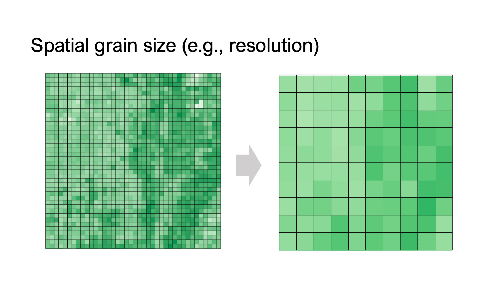
When we change the spatial resolution of a pixel, we change the number and type of elements (for example landcover types) that compose it. This highly impacts outcomes where we attempt to classify pixels based on their composition.
![]()
Challenge: Why does spatial resolution matter?
Case study
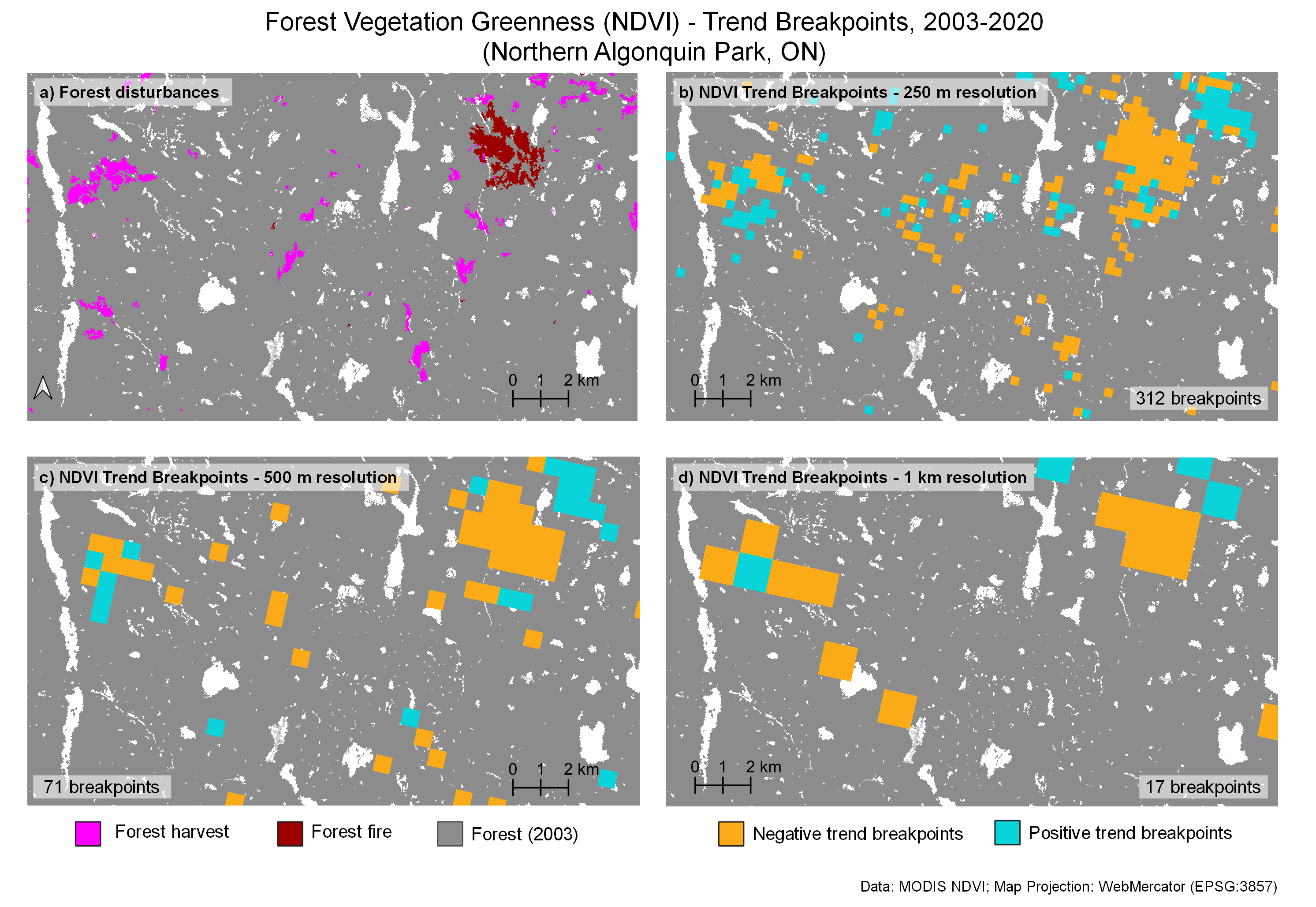
In the figure on the top right, we show two major forest disturbance agents (panel a) and the results of a geo-spatial trend analysis (panel b to d) over a relatively small study area (26,000 ha) located along the northern boundary of Algonquin Park. The vegetation greenness of forests, as measured by the Normalized Difference Vegetation Index (NDVI), shows many trend breakpoints over an 18-year long period (2003-2020). Trend breakpoints refer to structural changes in the trend line of a measurement. Trend breakpoints can be positive or negative and can result from forest natural and anthropogenic disturbances.
When using MODIS derived NDVI at a 250 m resolution (panel b) we find 312 different trend breakpoints in the data. Most of these are negative breakpoints (orange color pixels), meaning that some forest areas have experienced important decreases in greenness at some particular point in time. However, there are also some forest areas that have seen significant increases (turquoise color pixels) in greenness at a particular point in time. When a 500 m resolution NDVI time series is used instead (panel c), the number of breakpoints drops to 71. Similarly, when a 1 km resolution NDVI time series is used (panel d), the number of breaks further decreases to 17.
Interestingly, not only does the number (and direction/sign) of forest pixels with trend breakpoints change depending on the resolution of the data but also the pixel locations over the study area. Some of these trend breakpoint pixels spatially and temporally overlap with forest harvest and fire events. The largest overlaps occur when using the finest spatial resolution (250 m) data. Thus, the spatial resolution of a dataset may influence the results obtained and in turn, the management decisions that may arise from them.
Challenge: Why does spatial resolution matter?
Best practices and opportunities
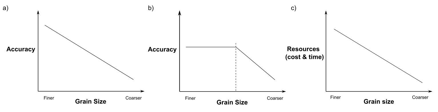
In cases where different data resolutions are available, the recommendation is to use data at the finest spatial resolution to ensure that potentially relevant ecological patterns are not missed.
Even though, fine scale data usually leads to improved accuracy of models (Fig. a & b), there are several constraints such as data availability, data storage, computing power, time, and financial resources (Fig. c). Finer grain size (i.e., smaller pixel size) usually leads to improved accuracy but some processes actually plateau at a certain resolution and there is no need to go finer. This is often used as a baseline for future studies. Higher resolution often comes with higher cost and time and hence, it is important to identify the most optimal point for a given study based on resources available.
Challenge: How to aggregate data to scale up?
[under construction note]
Introduction
In addition to the resolution, boundaries used to aggregate smaller scale data may influence the visual assessment of ecosystem service supply and demand information and relationships.
Challenge: How to aggregate data to scale up
Case study
Pollination supply and demand aggregated to watersheds (left) tend to show ecosystem service surplus (i.e. higher ratios) at areas with little demand, while the supply and demand relationships represented at 3km grid cells (right) can help identify more precisely high demand areas that could benefit from more agricultural support.
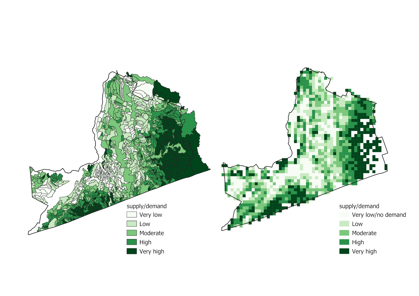
Figure showing pollination data aggregated to watersheds (left) or pixels (right)
Challenge: How to aggregate data to scale up
Best practices and opportunities
Careful consideration of the aggregation, reporting, or zonal unit by assessing variance or representativeness (i.e., percentage of outcome agreement and disagreement between scales).
Consider the effects of aggregating information at the ecologically meaningful level into socially meaningful or management scale.
Challenge: How to consider non-linearities?
[under construction note]
Introduction
Often we assume a relationship between two variables is linear; however, if we increase the spatial extent we may see a nonlinear relationship appear. This is important, because we often predict in areas outside of where we sample. If we assume a relationship is linear, when it is not, then our extrapolations will be incorrect.
Challenge: How to consider non-linearities?
Case study
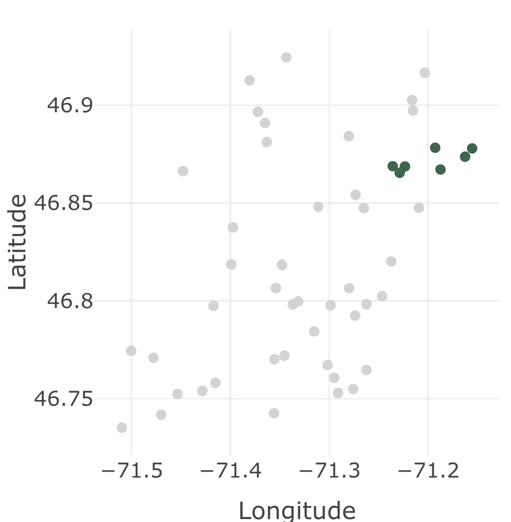
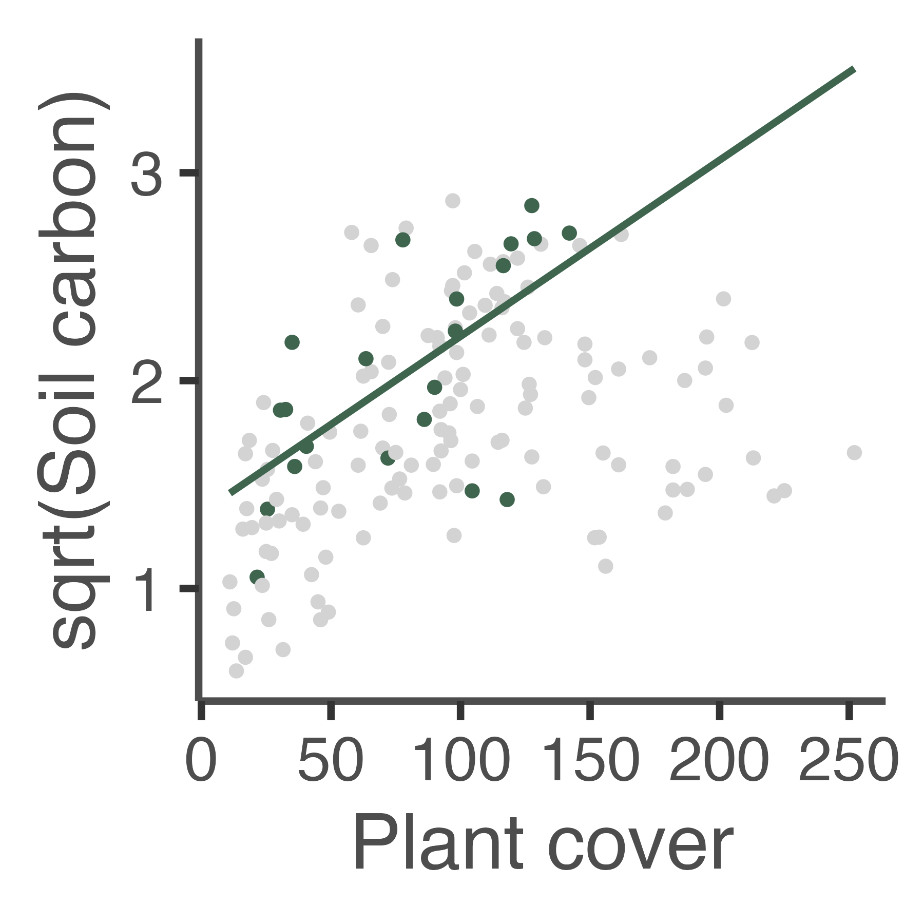
In this case study, we show the relationship between soil carbon and plant cover in vacant lots in Quebec city. Plant cover can be greater than one in densely vegetated vacant lots when leaves overlap. In this study, vacant lots were carefully selected to represent the entire range of plant cover.
However, a less careful scientist, could have selected only a subset of these vacant lots (green dots, map on left). The relationship between soil carbon and plant cover only within this subset (green dots, middle panel) is linear and would lead to an incorrect extrapolation to the whole study region (gray dots, middle panel).
When using data from the whole study region (e.g., increasing the spatial extent), we find that the relationship is actually non-linear (panel on right). In vacant lots with high plant cover, other factors (e.g., soil type, land use history, etc.) might be needed to better explain the variability of carbon.
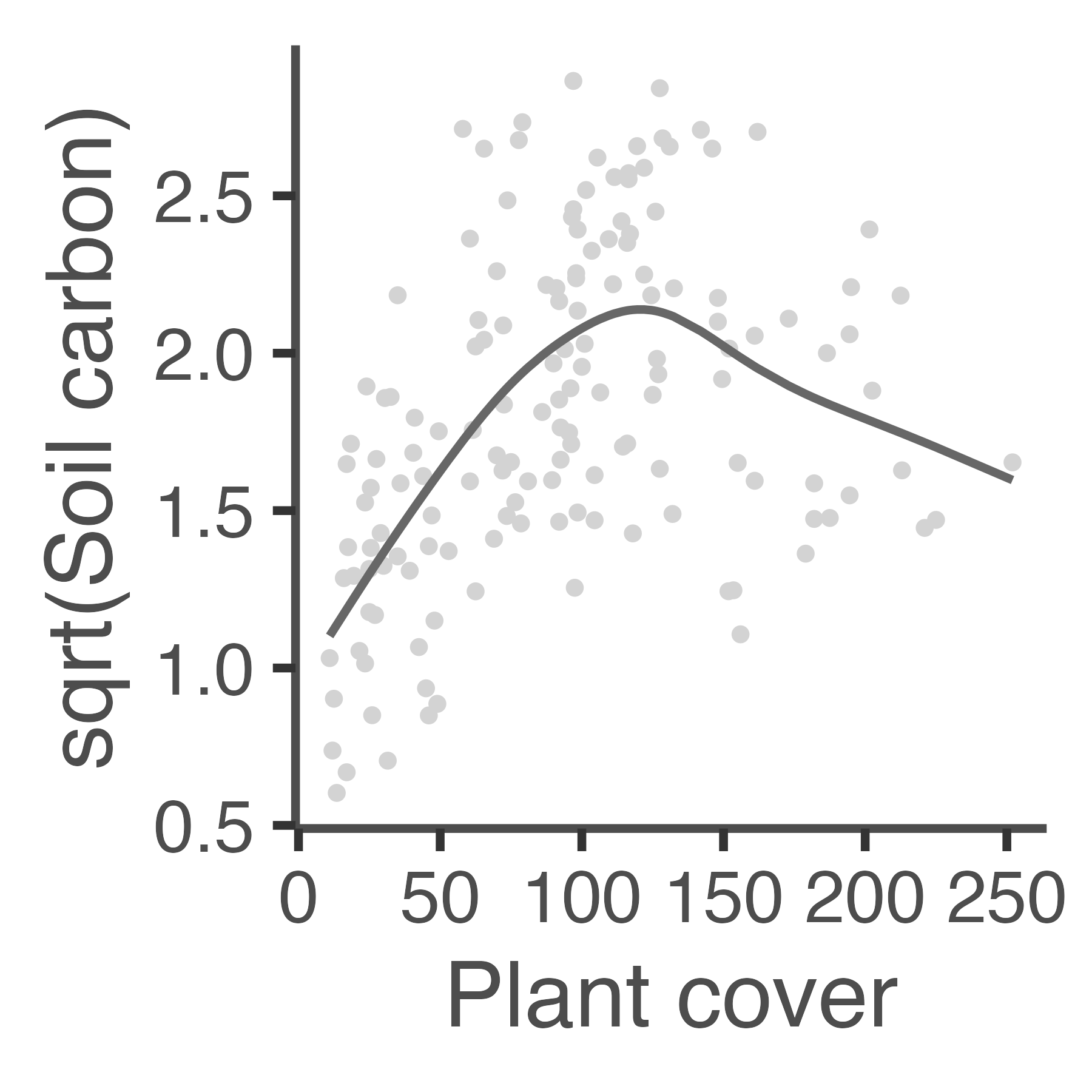
Data source: Poliana Mendes [add reference to submitted paper]
Challenge: How to consider non-linearities?
Best practices and opportunities
If funding and time allows, sample across a larger spatial extent to capture the full range of each variable.
When extrapolating outside of the original study region consider whether the new study region’s environmental variables are within the same range as the original study. If not, consider whether a non-linear relationship is likely.
Seasonality can also result in nonlinear relationships between a variable and time (e.g., temperature). To account for variables that vary across a year, we may need to monitor at the same time each year or more frequently within the year. Phenological changes are shifting with continuing climate change, which makes monitoring more frequently over time especially important.
Challenge: How does the monitoring time period influence outcomes?
[under construction note]
Introduction
Often we use time series analysis to understand whether an ecosystem property or service is changing over time. The temporal extent (e.g., time frame or period) of the monitoring data can affect outcomes. For shorter time-series or time-series with high variability, we may not have a correct historical baseline to detect change. For example, if monitoring data does not extend far enough into the past, then an insignificant trend could be interpreted as evidence for stability or no effect, when in reality the system might already be in a degraded state.
Challenge: How does the monitoring time period influence outcomes?
Case study
In this example, we show how Chinook salmon populations are changing in the Salmon river, British Columbia, Canada. In this region, Chinook salmon are important for the way of life for Indigenous communities, the economy, and the environment. Here, we show differences in trend significance depending on the start of a monitoring program. For example, if salmon monitoring only started 10 or 20 years ago (click on “since 2010” or “since 2000” buttons), then no significant downward trend would have been detected. However, if we begin our time-series analysis in 1984, then we see a significant downward trend: slope = -0.046 and p-value < 0.001.
Data Source: Fisheries and Oceans Canada. 2021. NuSEDS-New Salmon Escapement Database System. Retrieved here on Jan 13, 2022.
Challenge: How does the monitoring time period influence outcomes?
Best practices and opportunities
Even when monitoring data are available for 30+ years, we know ecosystems have been changing over centuries. For example, current observations of salmon in the Salmon River are very different from historical reports.
“In the grey of early morning I was aroused by a commotion, and found the river full of sockeye running upstream. I put in an oar and felt that the river was half fish. The increasing light soon showed that it was red from bank to bank. Then a stampede or panic occurred, and the salmon came surging down, but the river was so full of ascending fish that they blockaded and made a great flat wriggling dam. So jammed were they that they crowded out, and were rushed up the sloping banks out of the water.” -David Salmond Mitchell, fisheries officer 1905
Source for quote: Burt DW and Wallis M. 1997. Assessment of salmonid habitat in the salmon river, salmon arm. Department of Fisheries and Oceans. Vancouver, B.C.
[fix blockquote style]
When appropriate historical baselines are unavailable, comparisons can be made with an equivalent reference site. However, in the age of the anthropocene, finding an appropriate reference site can also be challenging. Therefore, when reading papers and reports, we suggest to critically evaluate how baselines and reference sites were selected and how these choices could impact outcomes.
Challenge: Spatial, temporal, & scale mismatches
[under construction note]
Introduction
In some cases, the supply and demand for an ecosystem service do not overlap in time or space. The interactions and processes connecting the source of supply and its demand are often called “ecosystem service flow”.
No-overlap between supply and demand can occur due to mismatches in space, time, or scale.
Challenge: Spatial, temporal, & scale mismatches
Case Study
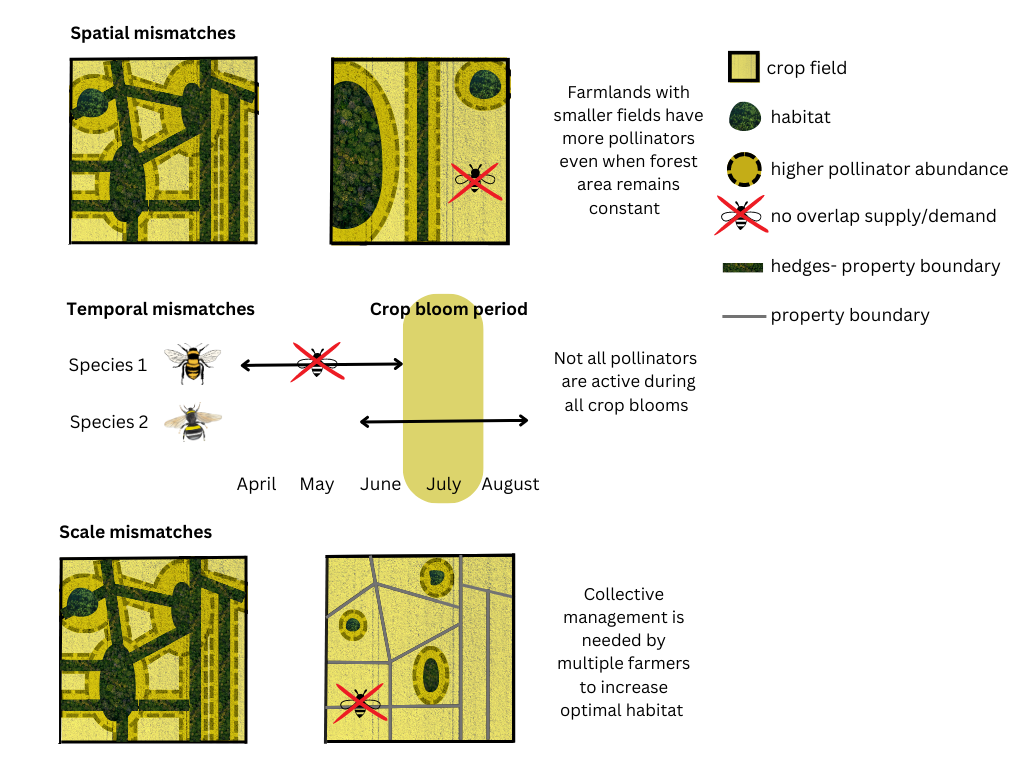
Here, we provide examples of when supply and demand don’t overlap due to mismatches in space, time, or scale using the ecosystem service of pollination as an example.
-
Spatial: when we change the spatial extent of a study, we might miss sources of ES supply or ES beneficiaries. The figure in the left shows an example: Even when habitat for pollinators is constant across two landscapes, farmlands with smaller fields often have higher pollinator abundance, showing the influence of the spatial scale on the supply of pollination.
-
Temporal: Not all pollinators are active during all crop bloom seasons. As climate change continues, the phenological response of crop blooms and bee emergence may differ, which may result in greater temporal mismatches.
-
Scale mismatch: The whole process of pollination, from the location of pollinators' habitat, their feeding dynamics and flying range requires a minimum spatial extent and configuration of the habitat that might exceed that of a single farm. In other words, one farmer may not have have enough land to set aside to support pollinator habitat, or an optimal configuration of pollinator habitat, but working together multiple farmers would. So incentives that encourage cooperation among farmers, may be more successful than incentives that support a single farmer increasing bee habitat. This is because the scale of management (a single farm) is too small in spatial extent to match the scale of the process of pollination.
Challenge: Spatial, temporal, & scale mismatches
Best practices and opportunities
[This section will be updated after the AGM.]
Some topics we will consider including:
- Consider the serviceshed and define the beneficiary
- Cross beneficiary comparisons
- Assess the benefit gap
- Consider configuration in addition to extent of habitat areas
Challenge: The future is not like the past
[under construction note]
Introduction
When researchers study ecosystem services they are often interested in how land uses have changed in the past and how they might change in the future, and as a result how the services provided shift in location and amount. More generally, just as researchers choose the spatial extent and grain for their studies, they also choose the temporal extent and grain, asking questions such as: How far back in time should I go? Do I only care about annual changes, or do I want to know about changes within years?
Some ResNet projects have studied historical changes over several decades or centuries (e.g., Venter et al., 2016; Sherren et al., 2021), and in one case back five thousand years (Hillis et al., 2022). Similarly, some projects are focusing on possible future changes in ecosystem services resulting from human actions. For example, one research team is studying restoration of vacant lots in Quebec City (e.g., Rioux et al., 2019; [XXX get suggested reference from Poliana XXX]). Another group is studying the possibility of agriculture in the Northwest Territories 40-60 years in the future (Krishna KC et al., 2021; Lemay et al., 2021).
The tools and approaches for assessing ecosystem services in the past are not the same as those for projecting into the future – and the methods for studying the recent past or the near future are not the same as those for understanding times more distant from the present. For example, global carbon emissions are well known in the recent past, but the future trajectory is very uncertain and strongly depends on human actions. Especially over large areas, data from satellite sensors has been essential to understanding changes over time, yet accessible satellite data only extend back to 1972 (ref NASA). Before that, other data sources such as aerial photos and historical records, and methods, such as participatory GIS methods with knowledge holders (e.g., Brown and Fagerholm, 2015), must be used. And when studying the social aspects of ecosystem services, for example through interviews, we can only obtain input from people who are still alive.
This creates significant challenges when scaling up in time, that is, moving from a short duration study to a longer time period, and when combining assessments of past and future services.
Challenge: The future is not like the past
Case study
The following case study illustrates some of the challenges with scaling up in time, and the differences between scaling up information from the past and predictions for the future.
People obtain ecosystem services when they harvest wild plants (such as berries or mushrooms) from forested land. Such harvests go back hundreds of years in Canada, first by Indigenous peoples, then by settlers and now by a mix of different users (Kumar et al., 2019; MacKinnon et al., 2015; Turner, 2020). With the adoption and spread of industrial agriculture, and the reduction in forested land, the relative importance of such food sources in Canadian diets has dropped.
Here, we create a “snapshot” of the present – to understand the ecosystem services from harvesting wild plants found in Canada’s forests. For this case study, we have focussed just on the Montérégie region of Quebec, but have considered the methods used to scale up in time – either back into the past or forward into the future. [Note: this case study excludes trees harvested for timber or fuel wood, and maple syrup.]
This region has evolved dramatically over the last five centuries, with changes in control of land from Indigenous people to settlers, growth in human population, shifts in land use, forest clearing, establishment of increasingly industrialized agriculture, urbanization and development of an extensive road network.
‘[To visualize these changes, we will show three images of forest cover for the Monteregie: historical (pre-European), recent past, and current. Potentially with a sliding control so viewers can switch back and forth between them.]’
Challenge: The future is not like the past
Best practices and opportunities
This case study highlights the potential role for several best practices. These include:
-
Finding ways to combine information from multiple sources. This will be particularly important when scaling up to longer durations, when a greater variety of data sources and methods need to be used. For example, unconventional sources (e.g. historical photographs, old herbarium records) may be helpful. Bayesian methods can help assign weights to different sources, while retaining estimates of the uncertainty and flexibility in terms of the evolution of functional relationships.
-
Using mapping techniques, such as participatory GIS methods, to identify where current beneficiaries are in relation to the locations and services they value.
-
Recognizing that the future is not simply a linear extension from the past. This might mean deliberately including decision makers and beneficiaries of ecosystem services in research related to the future, through techniques such as scenarios. It might also include modelling human learning and adaptive management as part of predictions. Some researchers have recommended considering longer time extents than the focus of current decisions (e.g., Lyon et al., 2022).
Challenge: Model comparisons
[under construction note]
Introduction
Decision-making and research questions are meaningful at specific scales and often need scale-specific models.
Choosing the right size to study natural phenomena is hard for scientists (Oreskes et al., 1994). An appropriate scale determines how detailed and accurate their models are and how much area they can cover. The scale of a study significantly impacts the complexity, accuracy, spatial extent, and generalizability of the models (Brimicombe, 2010).
Researching a local scale or small proportion of the territory requires more complex analyses. Researchers need to consider more variables and their relationships to achieve a reliable approximation of the natural phenomena under investigation. Also, the identification of patterns could be more difficult. Furthermore, obtaining more detailed results demands more computational resources. Nevertheless, it should be noted that higher scales at a finer resolution do not always lead to higher accuracy (Brimicombe, 2010).
On the other hand, examining natural phenomena through regional or global studies may enhance comprehension. Coarser resolutions could lead to reduced complexity, simplifying inputs and outputs. Also, some relationships or patterns emerge to significant geographical extents due to noise reduction. Furthermore, Policymakers tend to favor regional and global scales, as they provide a broader perspective on reality (Brimicombe, 2010; Woolmer et al., 2008).
Challenge: Model comparisons
Case study
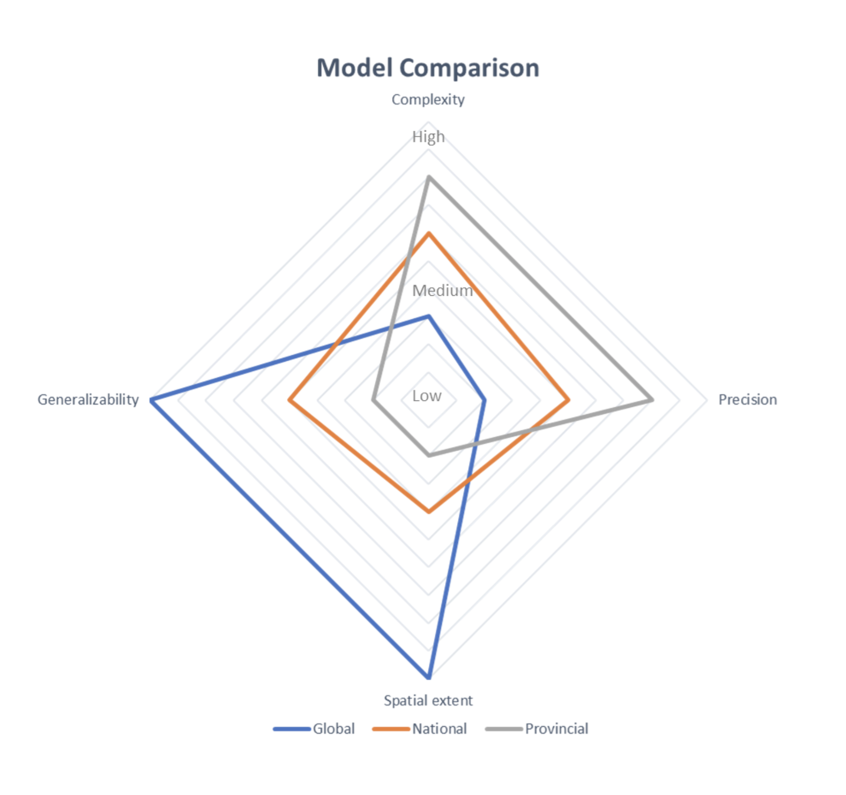
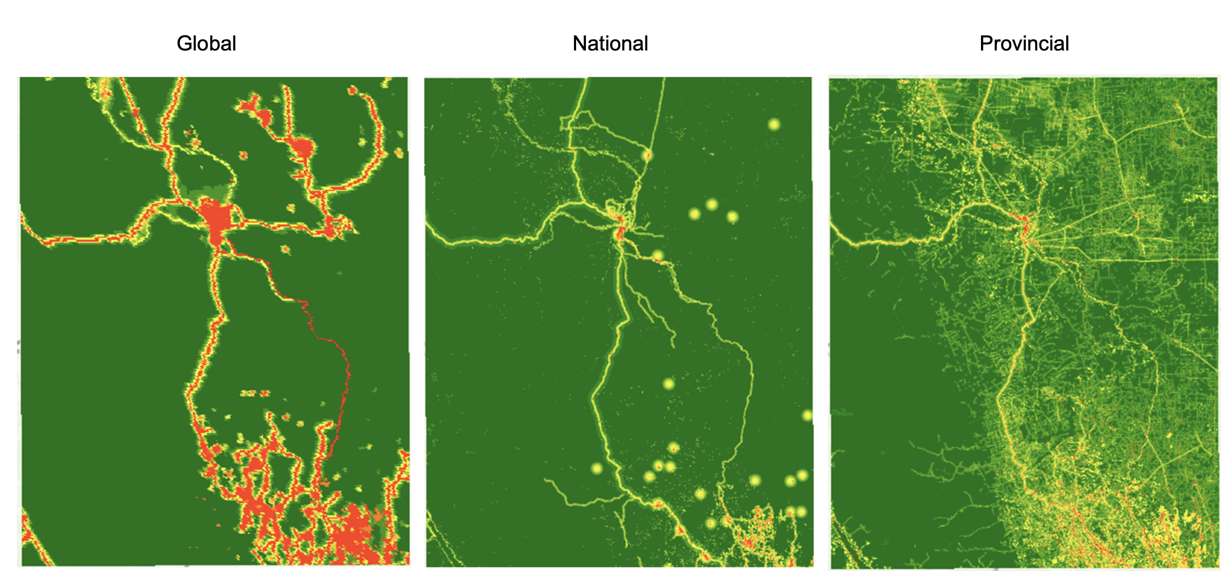
Here, we compared the Human footprint at three scales: Global (Williams et al., 2020), National (Hirsh-Pearson et al., 2022), and Provincial. The human footprint is a cumulative index that quantifies the extent and the intensity of human pressures on ecosystems and biodiversity.
This sample represents the state of human pressure in the northeast of British Columbia. From coarse (global) to detailed (provincial) resolution, we identify how roads are represented to different extents. Regarding complexities, with 8 mapped variables, the global model captures a broad perspective of human interventions in which roads and settlements are the most visible features. The map is improved with the national model, which integrates 12 layers, providing the first appearance of oil and gas infrastructure and mining. The provincial map, which incorporates 16 layers, shows a comprehensive state of the human footprint, including seismic lines, oil and gas wells, and infrastructure, even recreational features.
Challenge: Model comparisons
Best practices and opportunities
Models are very sensitive to the input data. The more accurate the input data, the higher the reliability of the model. Furthermore, model evaluation can be a complex process based on the nature and the extent of the phenomena. The larger the spatial and temporal scale of the phenomena, the more complex and challenging it can be to evaluate the model. Lastly, models are developed to be applied at a certain scale (spatial and temporal). A model acceptable at one scale might not be at another.
We suggest the following to improve reliability of models…
-
Clear and explicit criteria for every step of the evaluation
-
Document all decisions made to incorporate input data
-
Be clear about the purpose of the model
-
Conduct a sensitivity analysis to test the consistency of the model under a range of input parameters
Synthesis
[under construction note]
Synthesis of the spatial and temporal extents and resolutions of our different studies
We would like to synthesize the scales at which we work, inclusive of all ResNet related research projects. If you would like to be represented in our synthesis, please fill out our survey (1 response per research project).
Survey link: https://bit.ly/hqp-scale-survey
The purpose of this survey is to gain a better understanding of the spatial extent, spatial grain size, temporal resolution, and time period of research taking place within our network.
Your responses will be featured on our story map. For example, we hope to create a few scatter graphs showing the spatial and temporal scales at which we work (see example below). We will create a unique icon for each ResNet research study, and as the reader hovers over the icon, your name, title of your research project, and link for more information will be visible.
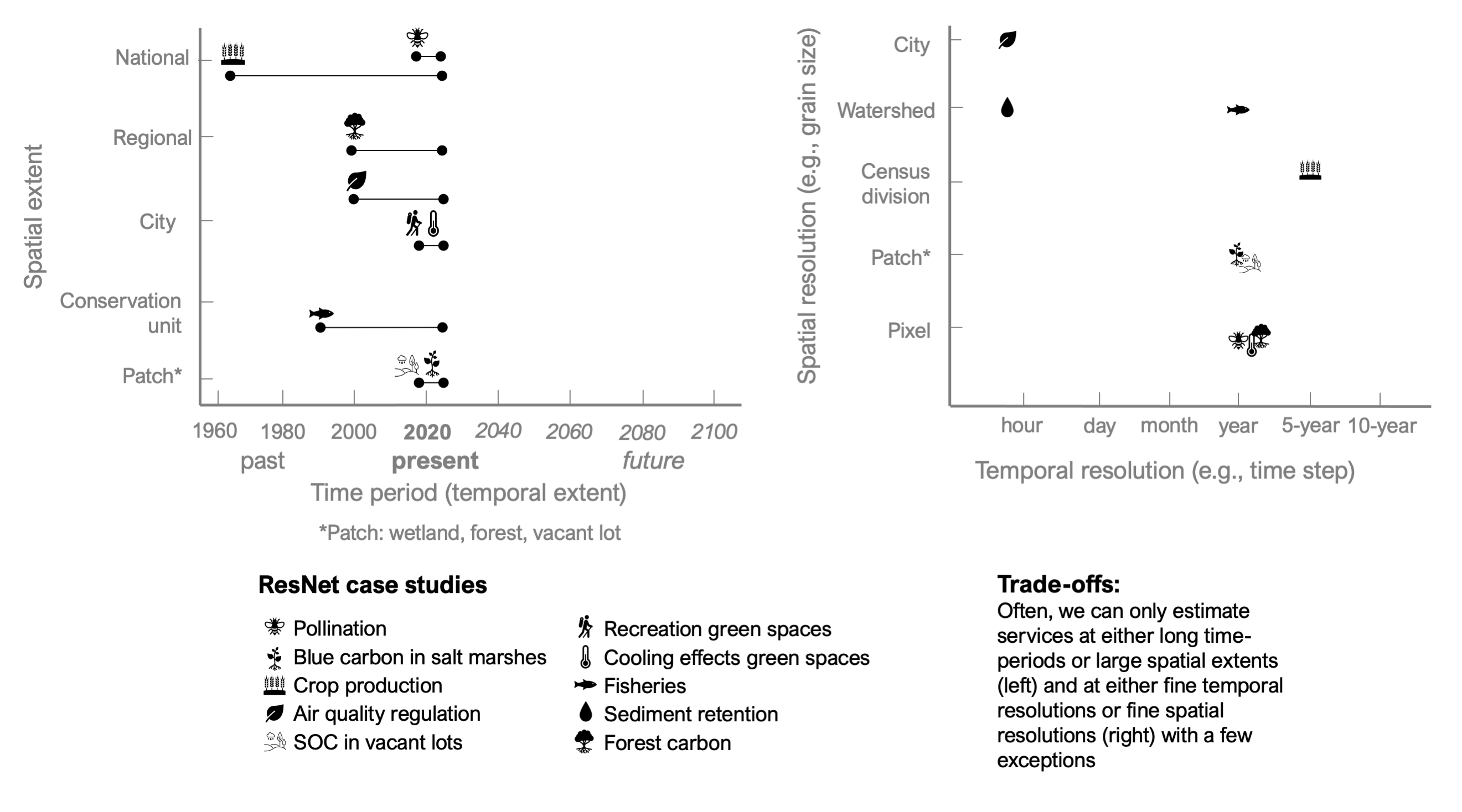
[These are placeholder images, we would like to make them interactive with additional information as the reader hovers over each icon.]
A landscape of scaling challenges
[This is placeholder text for a figure that synthesizes some of the challenges we discussed in the story map. We will hire an illustrator after the AGM.]
[We will also summarize a few key findings, which may include the following]
*Most of us study a specific aspect of this landscape. Only by talking more together can we better see how our studies are small pieces that fit together into a bigger picture.
*We found ourselves repeating one best practice over and over again: the need for modelers to talk more with field ecologists and local stakeholders.
Glossary
[under construction note]
Glossary of terms and definitions
[This section is under construction. References are going to be included in a later stage. Please feel free to suggest any extra definitions and/or terms.]
List of terms we will likely need to define and simple definitions
Ecosystem Service (ES): there are many similar, complementary and even contested definitions of ES. Ecosystem services are sometimes broadly defined as the benefits people obtain from nature [1], and more specific as the all the biophysical and social conditions and processes by which people obtain direct or indirect benefits from ecosystems [2, 3]. As a controversial concept, many frameworks have attempted to improve this definition to make it more clear and inclusive [4,5,6].
Ecosystem services supply, demand and flow:
Extent: see spatial and temporal extent definitions below.
Grain: Grain refers to the smallest or finest unit of measurement in a given data set.
Indicators:
Landscape Models: A model is an abstract representation of a system or a process. When describing or analyzing an ecological process, it is almost impossible to account for all the variables, interactions, feedback loops, inter-dependencies, etc. among ecosystem components, given the limited basic information available for analyses and processing capacities of computers [6,7].
Trade-offs: Trade-offs occur when the provision of one ES is reduced as a consequence of the provision or use of another ES. For example, carbon storage and sequestration is in trade-offs with timber extraction.
Pixel:
Patch: A region, a portion of surface that differs from its surroundings (e.g a patch of forest differs from a patch of agricultural fields). From a computer modelling perspective, a patch is a contiguous group of cells with the same class or category.
Resolution: Is the precision of a measurement. In the context of spatial analysis, resolution refers to the level of detail at which geographic data is represented. In other words, the resolution determines the smallest object that can be identified as a separate entity on a map or image
Spatial extent: Geographical size and boundaries of the study area.
Temporal extent: Duration of time covered by a process, or a study. It is defined by a specific time period.
Watershed:
References:
[This section is under construction. We will standardize and alphabetize at a later time. Also we are still collecting references from all sections, as some are still under construction]
Brimicombe, A. (2010). GIS, Environmental Modeling and Engineering. CRC Press.
Hirsh-Pearson, K., Johnson, C. J., Schuster, R., Wheate, R. D., Venter, O., & Hirsh, K. (2022). Canada’s human footprint reveals large intact areas juxtaposed against areas under immense anthropogenic pressure. Https://Doi.Org/10.1139/Facets-2021-0063, 7, 398–419. https://doi.org/10.1139/FACETS-2021-0063
Oreskes, N., Shrader-Frechette, K., & Belitz, K. (1994). Verification, validation, and confirmation of numerical models in the earth sciences. Science, 263(5147), 641–646. https://doi.org/10.1126/science.263.5147.641
Williams, B. A., Venter, O., Allan, J. R., Atkinson, S. C., Rehbein, J. A., Ward, M., Di Marco, M., Grantham, H. S., Ervin, J., Goetz, S. J., Hansen, A. J., Jantz, P., Pillay, R., Rodríguez-Buriticá, S., Supples, C., Virnig, A. L. S., & Watson, J. E. M. (2020). Change in Terrestrial Human Footprint Drives Continued Loss of Intact Ecosystems. One Earth, 3(3), 371–382. https://doi.org/10.1016/j.oneear.2020.08.009
Woolmer, G., Trombulak, S. C., Ray, J. C., Doran, P. J., Anderson, M. G., Baldwin, R. F., Morgan, A., & Sanderson, E. W. (2008). Rescaling the Human Footprint: A tool for conservation planning at an ecoregional scale. Landscape and Urban Planning, 87(1), 42–53. https://doi.org/10.1016/j.landurbplan.2008.04.005
Beaudoin A, Bernier PY, Villemaire P, Guindon L, and Guo XJ. 2018. Tracking forest attributes across Canada between 2001 and 2011 using a k nearest neighbors mapping approach applied to MODIS imagery. Canadian Journal of Forest Research, 48: 85–93. https://doi.org/10.1139/cjfr-2017-0184
Environment and Climate Change Canada. 2021. National Inventory Report 1990–2019: Greenhouse Gas Sources and Sinks in Canada.
Natural Resources Canada. 2022. Forest carbon emissions and removals. Net carbon emissions in Canada’s managed forests: All areas, 1990–2019. Retrieved from https://www.nrcan.gc.ca/our-natural-resources/forests/state-canadas-forests-report/disturbance-canadas-forests/16502 on 22 July 2022.
Natural Resources Canada. 2021. Canada’s forests provide solutions to a changing world. The state of Canada’s forests. Annual report 2021.
Authors:
(Alphabetical order by surname)
- Miguel Arias
- David Bysouth
- John Clark
- David Ferguson
- Evan McNamara
- Poliana Mendes
- Peter Morrison
- Ehsan Pashanejad
- Peter Rodriguez
- Brittney Roughan
- Amanda Schwantes
- Hugo Thierry
- Gabriela María Torchio
- Ágnes Vári
- Yiyi Zhang
[[
Picture
Name
Associated university
Role in academia: PhD student, master student, postdoc,
Link to your website or google scholar (if you have one)
]]